Lesson 1: Working with terrain data and satellite imagery 1
1. Retrieval of DEMs
We will first acquire two global sets of DEMs: GTOPO30 and SRTM. The GTOPO30 DEM, with a resolution of approx. 1 km, is suitable for very broad-scale analysis or maps (continental or national level). The SRTM DEM has a resolution of approx. 90m and is therefore suitable for the regional to small national scale. Both datasets are provided in so-called tiles for quadrangles covering a certain area. They can be downloaded for free, but you can also get the tiles required for this lesson, along with the other data, from the download link given below. The files srtm_04_08.tif, srtm_04_09.tif, srtm_05_08.tif and srtm_05_09.tif represent the SRTM DEM, the file W180N40.DEM the GTOPO30 DEM.
Learn more about GIS and RS data sources
Download training data for Hawaii
2. Preparation of GTOPO30 and SRTM DEM
Both datasets are provided in geographic coordinates based on the WGS84 coordinate system and require similar processing steps. Therefore, perform the following tasks first with the GTOPO30 DEM and then with the SRTM DEM.
- If the area of interest is at the border between different quadrangles i.e., if more than one tile is required to ensure a complete cover, the tiles have to be mosaicked before further processing.
Learn how to mosaic raster maps in ArcGIS 9.3 and in ArcGIS 10
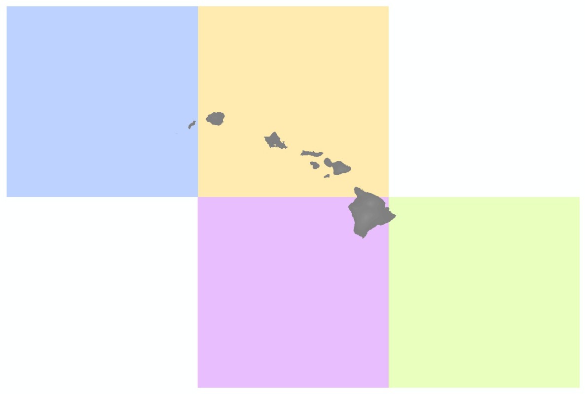
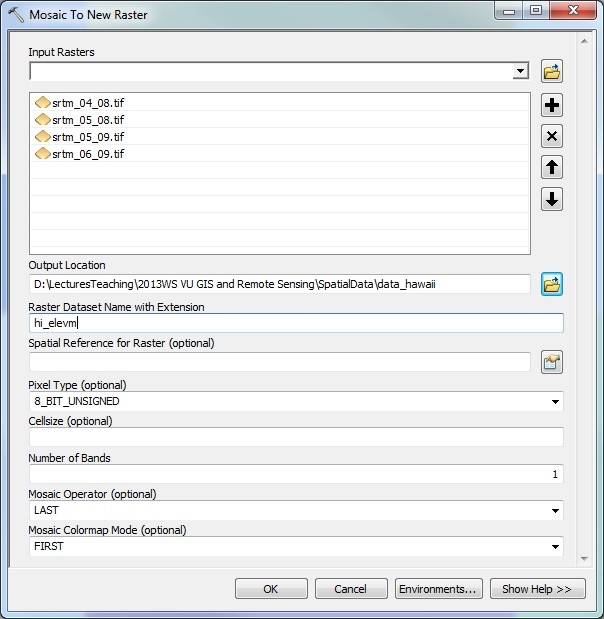
Tiles of the SRTM DEM (left, each tile is represented by one colour) and dialog box for mosaicking the tiles into one raster dataset (right). - The elevation unit used in the DEMs is metres. If you have a look at the range of values or if you query the map, you will see that the maxima go far beyond topographic elevation, reaching values above 50000. Such high values are used to identify no data areas, depressions or the sea. You should reclassify cells with such values to no data cells.
Learn how to reclassify raster maps in GRASS GIS 6.4, in ArcGIS 9.3 and in ArcGIS 10
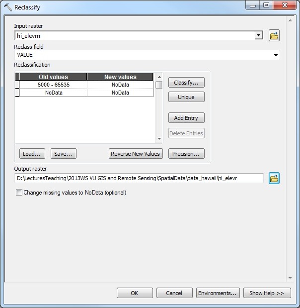
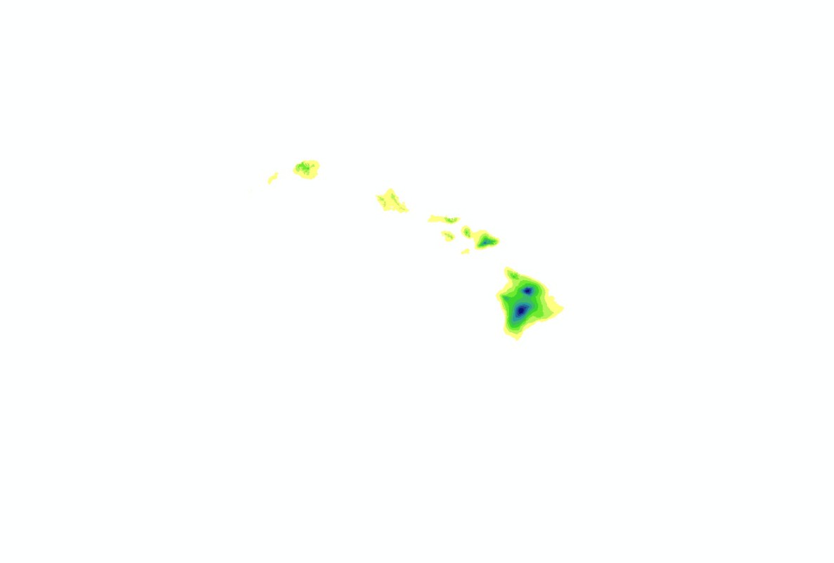
Dialog box for reclassifying the SRTM DEM (left) and reclassified dataset (right). - Even though most types of analyses can be performed on datasets with geographic coordinate systems (horizontal unit: degrees), it is strongly recommended to reproject the data into a projected coordinate system (horizontal unit: metres), preferably in UTM or - for very large study areas including multiple UTM Zones - World Mercator or another global reference system. In this case, use UTM Zone 5N.
Learn how to project raster maps in GRASS GIS 6.4, in ArcGIS 9.3 and in ArcGIS 10
View map of UTM Zones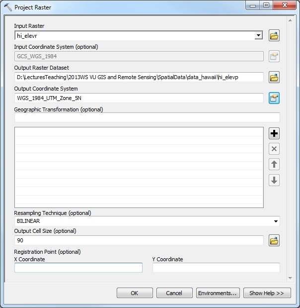
Dialog box for reprojecting the DEM to the UTM Zone 5N. - Finally, clip the dataset to an area slightly larger than your area of interest in order not to carry around unneccesary data slowing down the calculation processes. Along with the other data, you have downloaded an extent polygon for Hawaii hi_extent1.shp. Use this polygon for clipping the data.
Learn how to clip raster maps in ArcGIS 9.3 and in ArcGIS 10
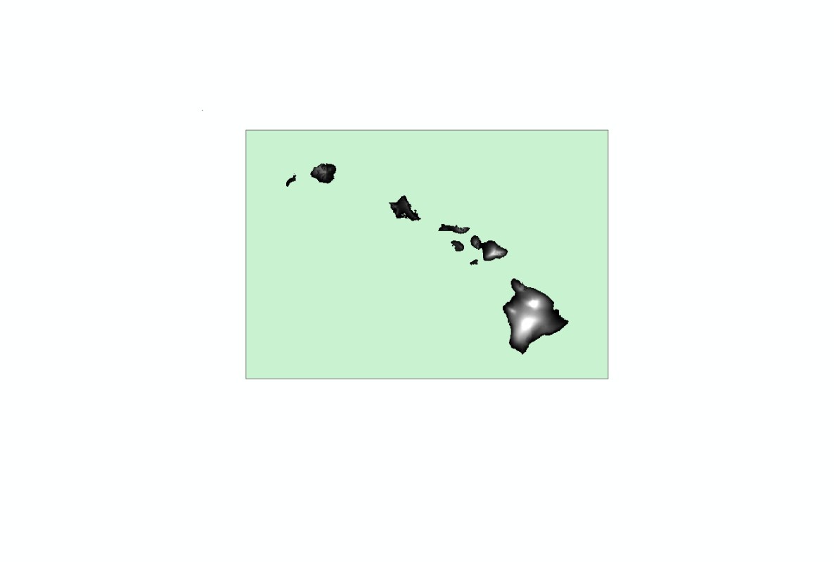

Reprojected DEM with clip polygon (left) and dialog box for clipping the reprojected DEM (right).
Now you have a dataset ready to be used for various types of analyses.
3. Terrain analysis with the GTOPO30 and SRTM DEMs
Most GIS software packages allow for a quick derivation of terrain parameters from cell neighbourhood computations in DEMs. Such parameters include hillshade, slope, aspect, curvature and some more. In addition, it is possible to create contour lines. Perform the following calculations first with the GTOPO30 DEM and then with the SRTM DEM. For all types of terrain analysis it is essential that the horizontal unit of the grid cells is the same as the unit used for elevation (usually metres).
- A shaded relief map or hillshade conveys a realistic impression of the terrain to the observer. Even though it cannot be used for any further analysis, it is an important component of GIS-generated maps and it allows for for a quick analysis of the plausibility of a DEM and for a visual interpretation of terrain characteristics. It is important to choose an appropriate sun angle - which does not necessarily correspond to a sun angle observed in reality, otherwise the terrain may appear inverted. Most people experience a realistic impression of the terrain if the assumed sun takes a northwest position.
Learn how to create a shaded relief map in GRASS GIS 6.4 in ArcGIS 9.3 and in ArcGIS 10
- Slope map: it represents the local slope in degrees, radian or percent, derived from the neighbourhood relations of the cells in the DEM.
Learn how to create a slope map in GRASS GIS 6.4, in ArcGIS 9.3 and in ArcGIS 10
- Aspect map: denotes the exposition of each pixel (north, northwest etc.)
Learn how to create an aspect map in GRASS GIS 6.4, in ArcGIS 9.3 and in ArcGIS 10
- The curvature map is the second derivative of elevation, or first derivative of slope.
Learn how to create a curvature map in GRASS GIS 6.4, in ArcGIS 9.3 and in ArcGIS 10
- Contour lines may be created from the DEM - like the hillshade, they are important for the design of maps rather than for analysis purposes.
Learn how to derive contours in GRASS GIS 6.4, in ArcGIS 9.3 and in ArcGIS 10
If you compare the datasets derived from the GTOPO30 and SRTM DEMs, you will note the different levels of detail and therefore different scope of the two datasets.
- The contour map is provided in the NAD83 coordinate system. As all our other datasets are in UTM Zone 5N, let's reproject this one also to this spatial reference. With some GIS software packages (e.g. ArcGIS), display and correct overlay would also work with different coordinate systems, but certain types of analyses would not.
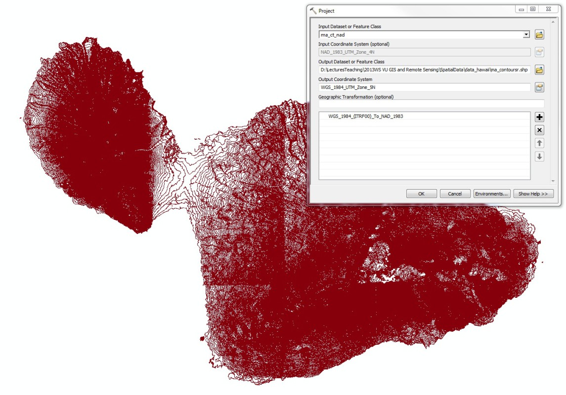
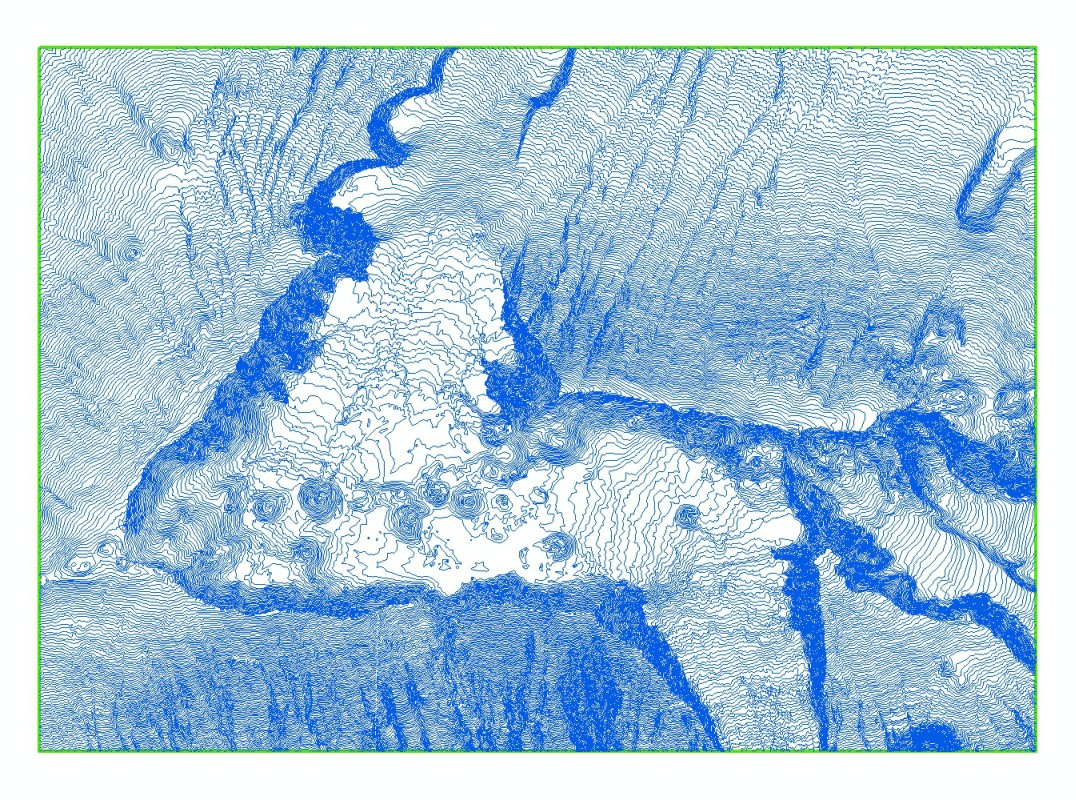
20ft contour lines for Maui with dialog box for reprojection into the UTM Zone 5N. - The dataset is very large and would require a lot of computing time, therefore we clip it to the extent we need. This only works properly if the data was reprojected before.
Learn how to clip features in ArcGIS 9.3 and in ArcGIS 10
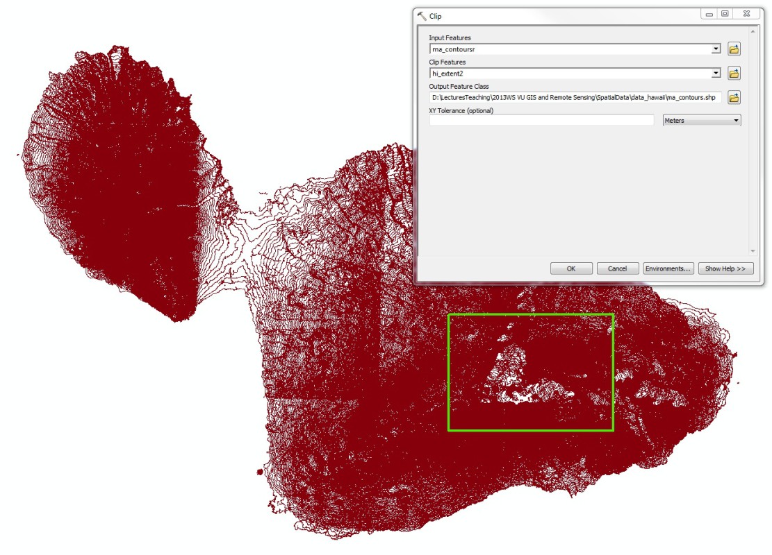
Reprojected contour lines with clip extent and dialog box for clipping (left), clipped contour lines (right). - Convert the line vertices to points. This is required for most feature-to-raster interpolation algorithms.
Learn how to convert line vertices to points in ArcGIS 9.3 and in ArcGIS 10

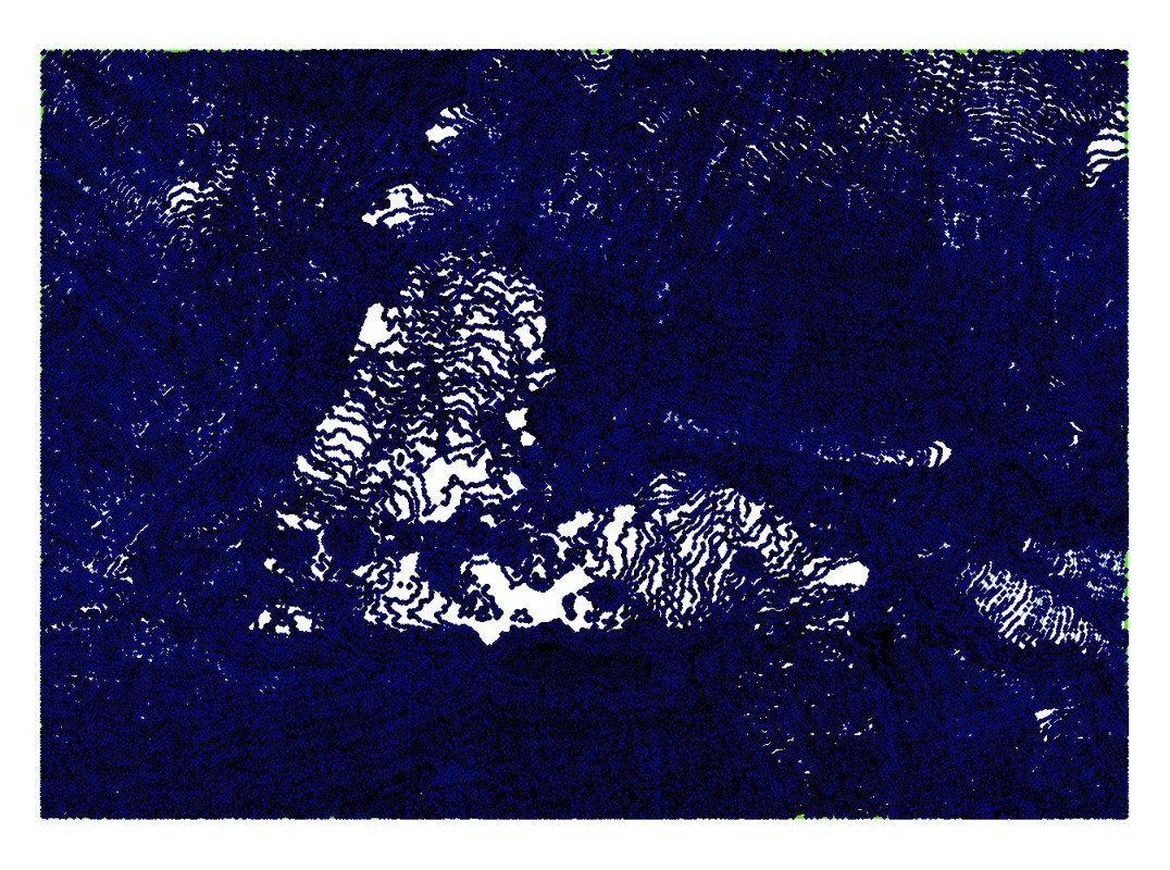
Clipped contour lines with dialog box for conversion of vertices to points (left), resulting point feature (right). - Interpolate the points to a raster map with 10 m resolution. Various functions to do so are available, also depending on the software you are using. All of them have their advantages, but also disadvantages.
Learn how to interpolate points to a raster map in GRASS GIS 6.4, in ArcGIS 9.3 and in ArcGIS 10
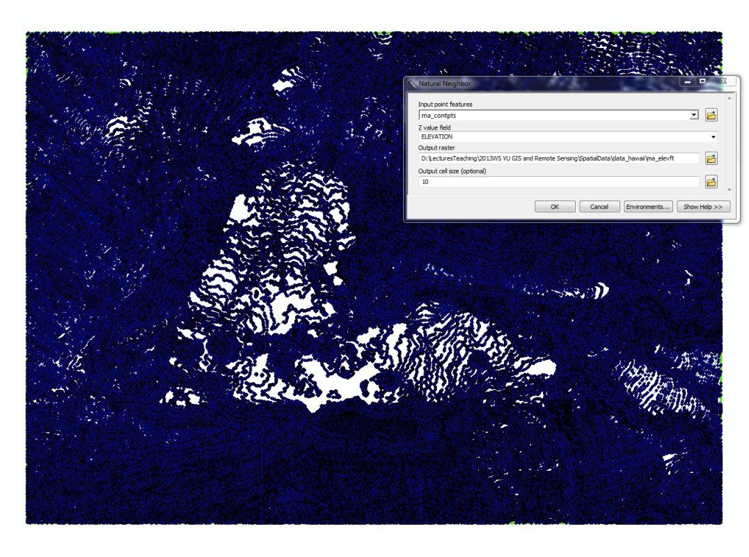
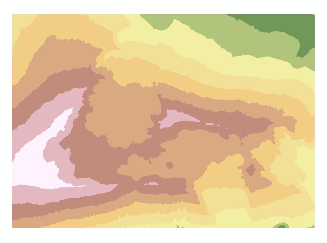
Points created from vertices of contour lines with dialog box for interpolation (left) and resulting DEM (right). - The best way to evaluate the elevation map is a hillshade. Create one and compare it to those generated from the other datasets.
- Create a true-colour composite image: this is done by combining the channels (or bands) 3, 2 and 1. Channel 3 covers the red spectrum, 2 the green and 1 the blue one. In the RGB mode, the combination 3-2-1 therefore represents the image in colours as perceived by the human eye.
Learn how to create a composite image in GRASS GIS 6.4, in ArcGIS 9.3 and in ArcGIS 10
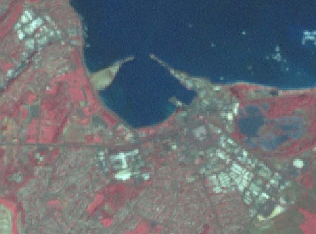
- Do the same with 4-3-2: Channel 4 is the near infrared channel where vegetation reflects very well and water not at all: this means that lush vegetation is represented in bright red and water in black. So called false-colour images are much more useful for many purposes than true-colour images since the blue channel does not contain a lot of signal.
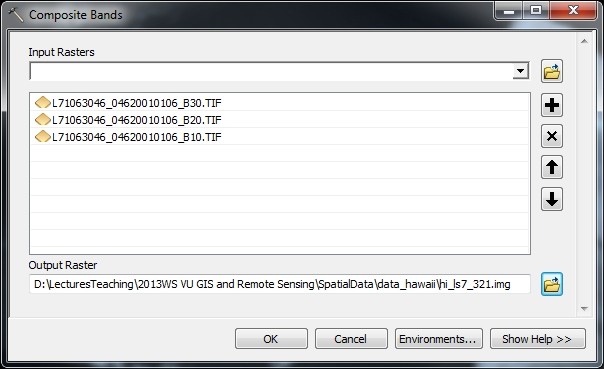
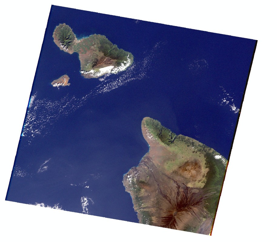
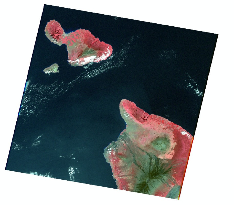
Left: dialog box for creating a composite image (the example shows a true composite with the bands 3 red, 2 green and 1 blue), middle: true-colour composite image, right: false-colour composite image (4-3-2). - Perform pan-sharpening: the channels 1 to 5 of Landsat ETM+ have a resolution of 30 m, the panchromatic channel 8 has a resolution of 15 m. Merging the 4-3-2 composite image with the panchromatic channel provides a higher spatial resolution (more detail in the resulting image) whilst maintaining the colour information.
Learn how to perform pan-sharpening in GRASS GIS 6.4, in ArcGIS 9.3 and in ArcGIS 10
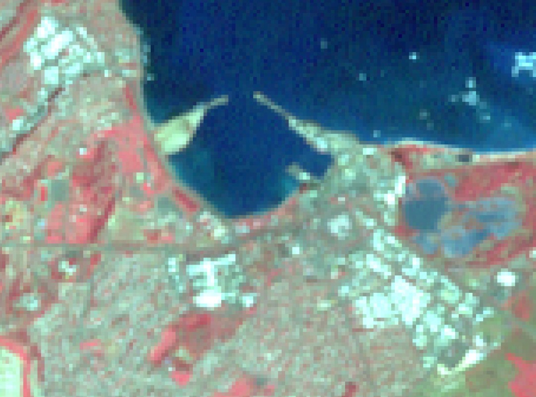
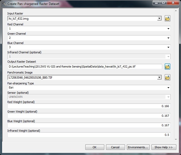
Landsat 7 false-colour composite of Kahului and Wailuku (Maui; left), dialog box for creating pan-sharpened image (middle), pan-sharpened image (right). - Clip all the channels of the Landsat image to your area of interest. When working with ArcGIS, you can use the batch mode to do so.
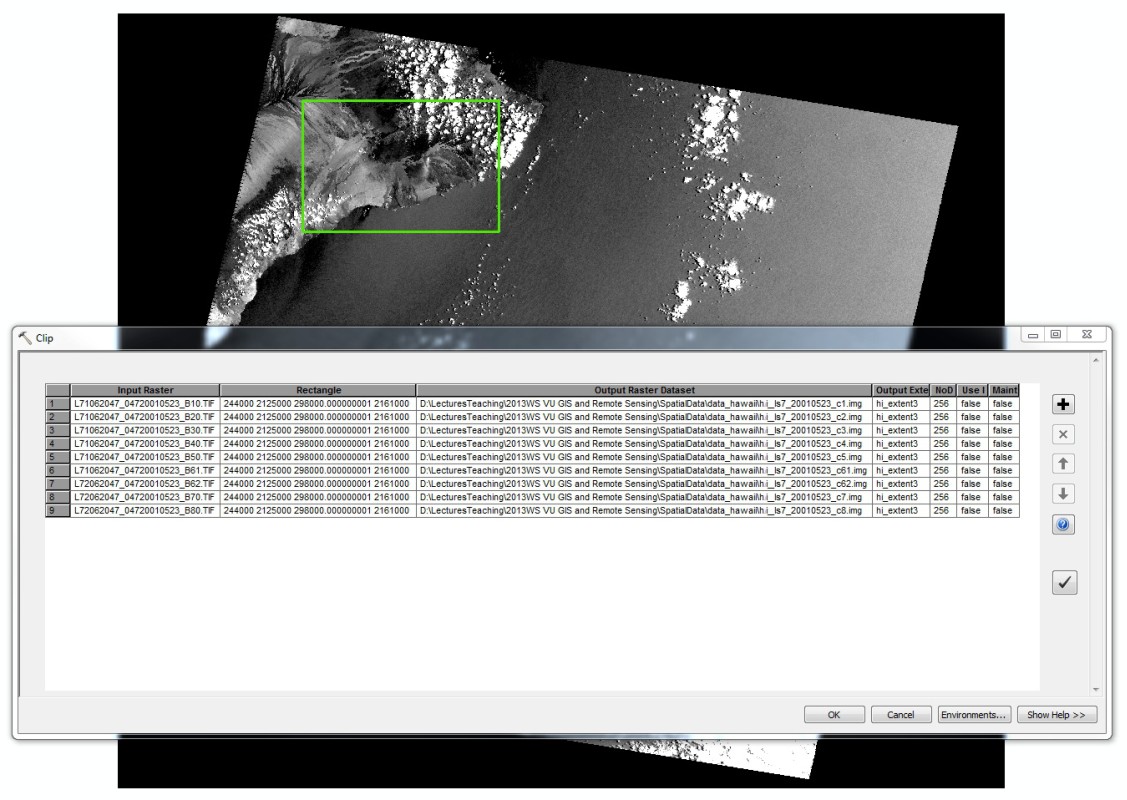
Batch clipping of Landsat 7 channels to the area defined by the shapefile hi_extent3.shp. - Create a true-colour composite image with the channels 3, 2 and 1 (just in order to get a visual impression of the study area).
- On our Landsat 7 image, clouds are well recognizable since no surface features have a comparably high reflectance. Query the values of clouds and areas without clouds, using channel 4, and try to find a reasonable threshold value. Then compute a new raster map where all cells above the threshold (clouds) get the value 1, all below (no clouds) 0.
Learn how to perform arithmetic calculations on raster maps in GRASS GIS 6.4, in ArcGIS 9.3 and in ArcGIS 10
- Expand the cloud areas in order to be sure to cover also cloud shadows which are hard to extract directly.
Learn how to expand areas with certain values in GRASS GIS 6.4, in ArcGIS 9.3 and in ArcGIS 10
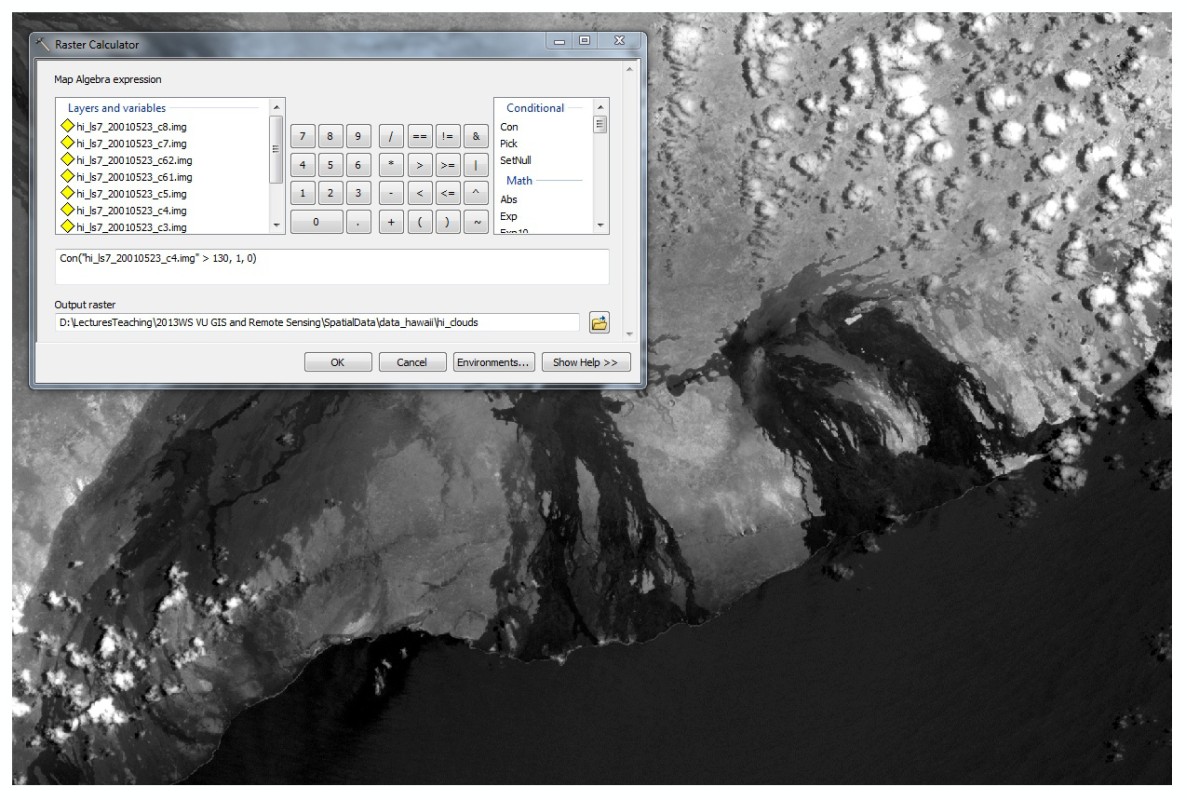
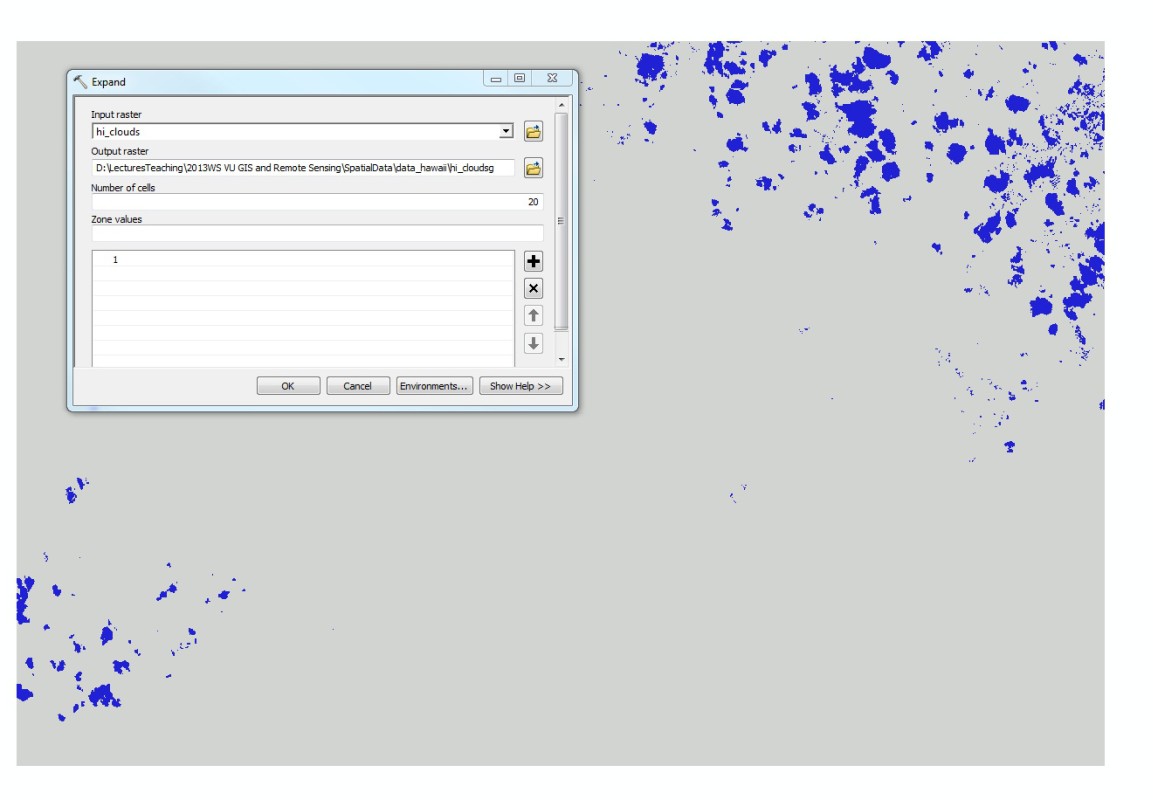
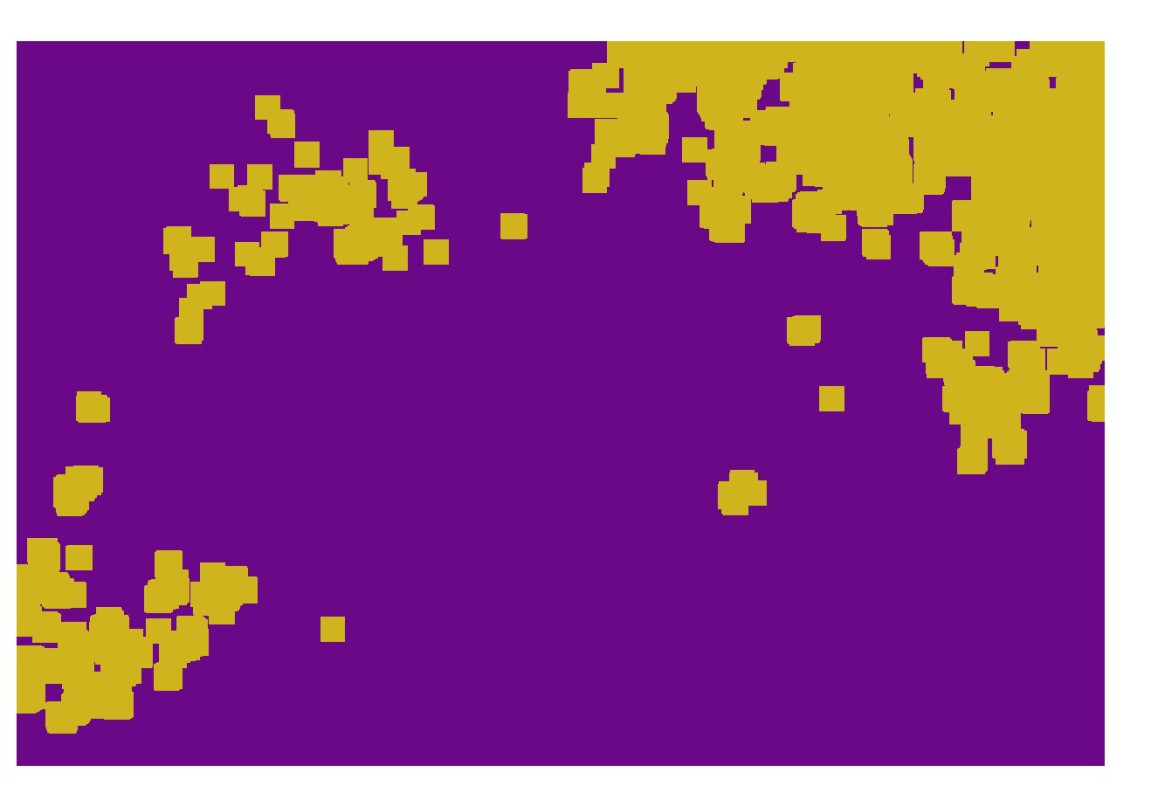
Dialog box for extracting the clouds from channel 4 of the Landsat 7 image (left), resulting binary raster map clouds/no clouds (middle), expanded cloud areas (right). - Next, identify those areas covered by the Pacific Ocean. Since it would be a non-trivial task to extract water surfaces from Landsat imagery, better use the SRTM DEM. Make sure to set the analysis extent and the cellsize to those of the satellite image before executing the raster calculation.


Dialog box for identifying areas covered by the sea (left), resulting binary raster map land/sea (right). - Now, compute the NDVI from the channels 3 and 4 (result values between -1 and 1). The NDVI map is often used to distinguish between various vegetation classes. In our case, we only try to establish a threshold between vegetation and no vegetation by querying the NDVI map. Using this threshold, compute a new raster map with vegetation=1, no vegetation=0, clouds/cloud shadows=no data and sea=no data.
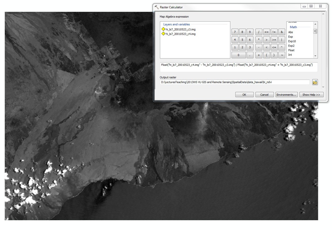
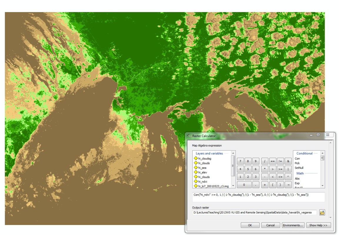

Dialog box for computing NDVI (left), NDVI map (middle; shades of brown: no vegetation, shades of green: vegetation) and dialog box for computing clean ndvi map, clean NDVI map (clouds and sea removed) with attribute table showing number of vegetated and non-vegetated raster cells (right). - Viewing the attribute table of the new raster, you can quantify the fraction of the study area being vegetated and the fraction not being vegetated.
- Visual interpretation of the channel will clearly indicate the location of active lava flows, if there are some.
- Try to find a lower threshold for active flows by querying the map. Active lava flows are characterized by raster cell values close to 255.
- Compute a map of active lava flows by assigning a value of 1 to cells with values above the threshold and 0 to cells below.
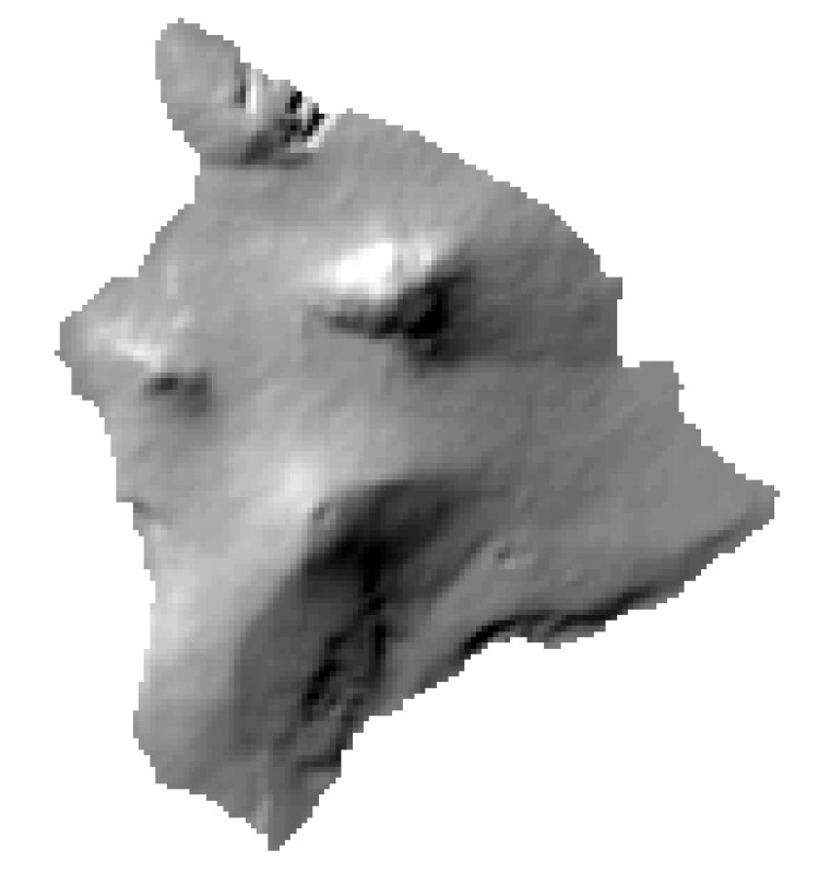
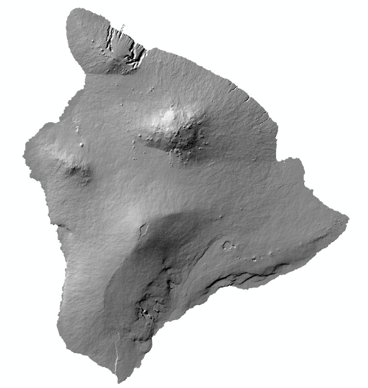
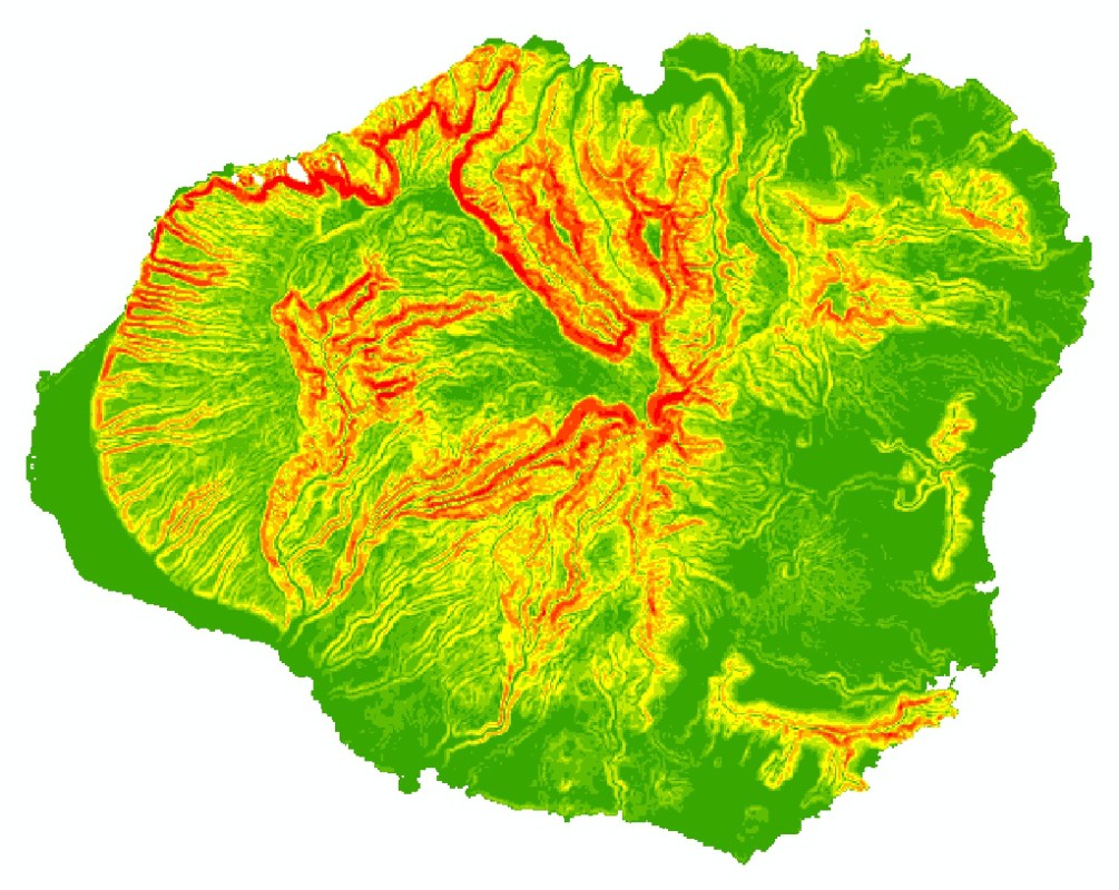

Hillshades created from GTOPO30 DEM (left) and SRTM DEM (left middle, both for Hawaii Big Island), slope map from SRTM DEM (right middle, for Kauai) and aspect map from SRTM DEM (right, for Maui and adjacent islands).
Combining elevation map, shaded relief and contour lines, you can produce a high-quality background for various types of maps. However, you can also use some of the datasets to derive a variety of further information - e.g., you can explore the statistics of elevation or or other terrain parameters over a specific area. Try to find the average and maxima of elevation and slope for each of the four main islands of the Hawaiian Archipelago: Kauai, Oahu, Maui and Hawaii Big Island. Use the SRTM DEM and the shapefile hi_islands.shp downloaded along with the other datasets.
Learn how to view zonal statistics in ArcGIS 9.3 and in ArcGIS 10
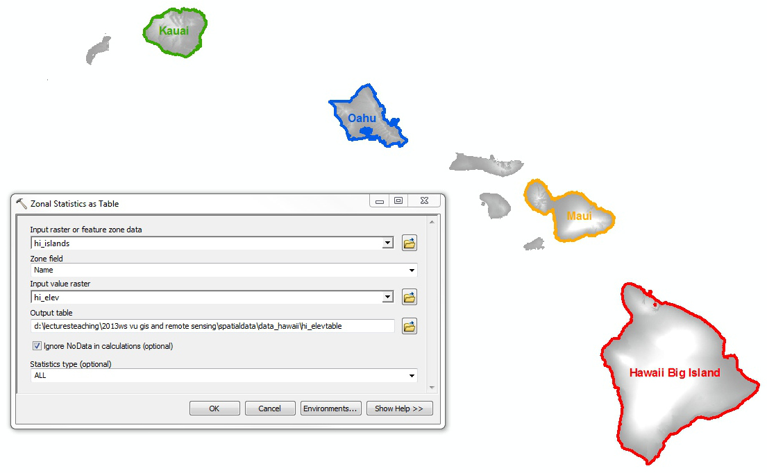
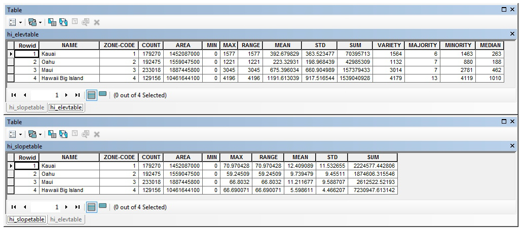
The four main islands and the dialog box for building zonal statistics of elevation (left), zonal statistics of elevation and slope (right).
4. Comparison with a higher-resolution DEM
High-resolution DEMs are often expensive and therefore only applicable for small areas. However, the governments of some countries, regions, provinces etc. provide higher-resolution DEMs for free. So does the state of Hawaii in cooperation with the United States Geological Survey (USGS). However, the data are not provided as raster, but as contour lines. You have downloaded the contour lines for the island of Maui ma_ct_nad.shp and the polygon feature of the area of interest hi_extent2.shp. You will create a higher-resolution DEM from the contour lines and compare it to the DEMs you have worked with before.
Try to interprete the landforms from what you see on the DEMs with different resolution. You will note the much higher detail recognizable from the 10 m DEM, compared to GTOPO30 and SRTM. But you will also recognize that DEMs in general only provide an incomplete picture of the earth surface - satellite imagery can add a lot of additional information.
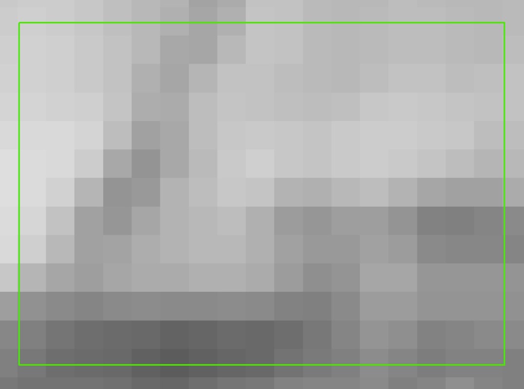
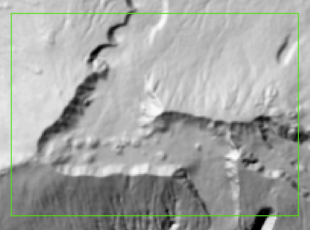
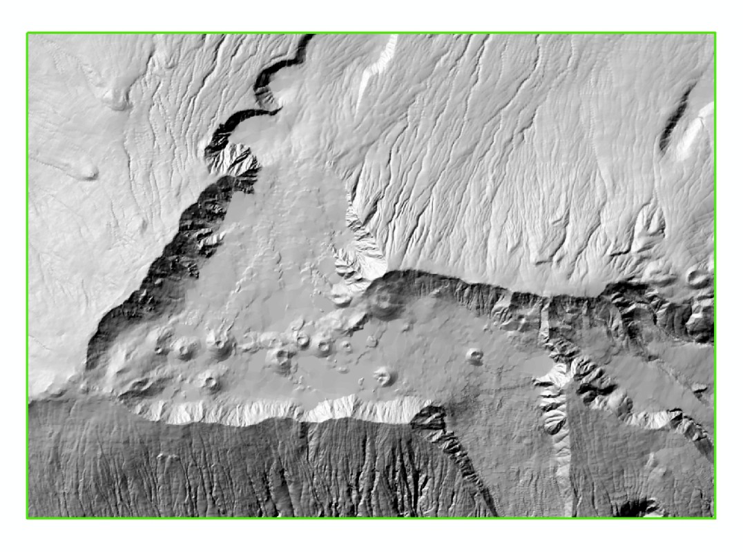
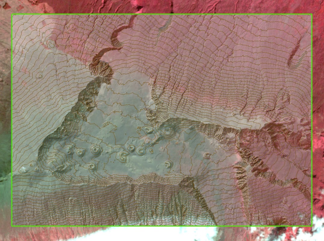
Hillshade created from GTOPO30 DEM (1 km cell size, left), SRTM DEM (90 m cell size, left middle) and the higher-resolution DEM derived from the contour lines (10 m cell size, right middle), overlay of the hillshade with the contour lines and a Landsat image.
5. Retrieval of Landsat ETM+ imagery
Retrieve the Landsat ETM+ image from January 6, 2001 from the Earth Explorer or use the downloaded image files L7*063046_04620010106_***.TIF. When having a first look on the files, you will find out that the dataset comes with various tiff files. All of them represent image channels covering a certain range of the electromagnetic spectrum. Channel 8 is panchomatic, meaning that it covers a broad spectral range. When opening one of these images e.g. with ArcGIS, you will find out that it is just a grayscale image with values ranging from 0 to 255, representing the reflectivity of the surface (land, water or clouds) within the spectral range covered by the corresponding image channel. Cell values of 0 indicate a very low reflectance, values of 255 a very high reflectance. Having a look at the spatial reference, you will notice that the image is provided in the UTM Zone 5N.
View data sources channels of Landsat sensors
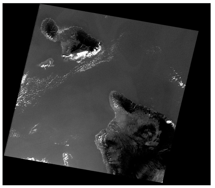
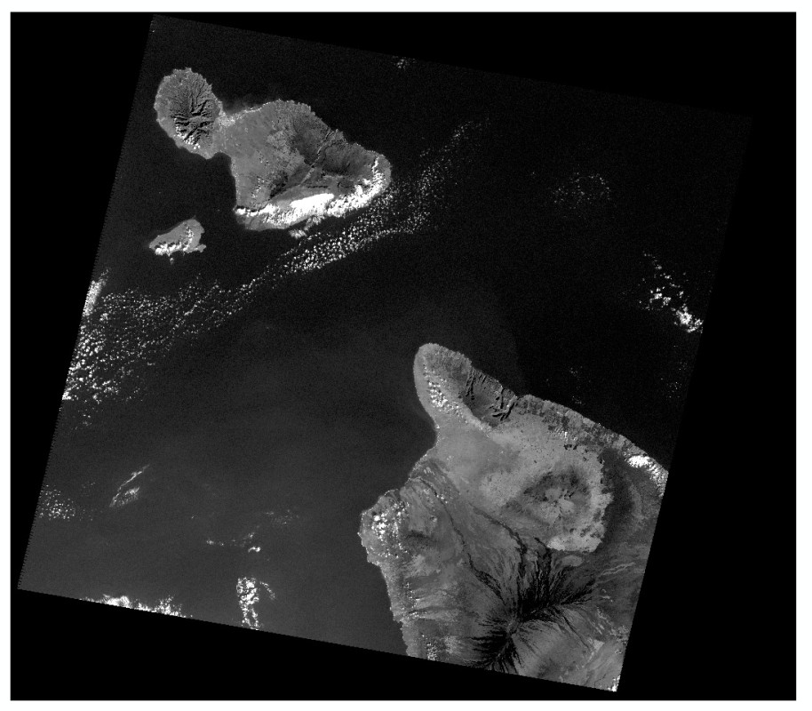
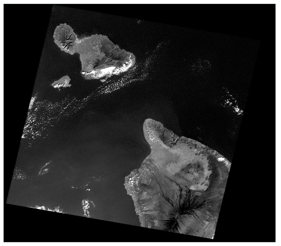

Landsat ETM+ channels 1 to 4 (from left to right), January 6, 2001.
6. Preparation of Landsat ETM+ imagery and visual interpretation
The information provided by each image channel for itself is very limited. Combining various channels can add substantial value to the imagery:
Now you can visually interprete the satellite imagery in combination with the DEM.
7. Quantitative interpretation of Landsat imagery
Combining the spectral signatures of different image channels, also quantitative analyses can be performed. In our case, we will first detect clouds and water and then compute the Normalized Differenced Vegetation Index (NDVI). We will move to Hawaii Big Island and use the area defined by the extent polygon hi_extent3.shp. The goal of this task is to quantify the fractions of vegetated and non-vegetated land within the extent polygon, excluding cloudy areas and the Pacific Ocean from the analysis. We will work with the image L71062047_04720010523_***.TIF.
In our case, this method allows to detect lava flows. In those moist, forested areas, disturbances (also landslides, debris flows etc.) are relatively easy to distinguish as most undisturbed areas are densely vegetated. In sparsely vegetated terrain (desert, high mountains), such a task would be much more challenging.
8. Detection of active lava flows
In the previous step, we have learned to find out where recent lava flows have occured in the last few decades. However, since such flows sometimes take place underneath the top layer of lava or are relatively small, it is not always possible to detect active lava flows using visible or near infrared channels.
Landsat ETM+ also offers channels in the thermal infrared spectrum. The signal they detect is a function of surface temperature, allowing for the identification of active lava flows. Use the file L71062047_04720010523_B61.TIF, representing the thermal channel of the Landsat 7 image from May 23, 2001.
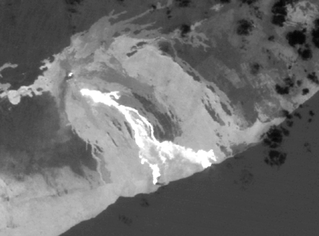
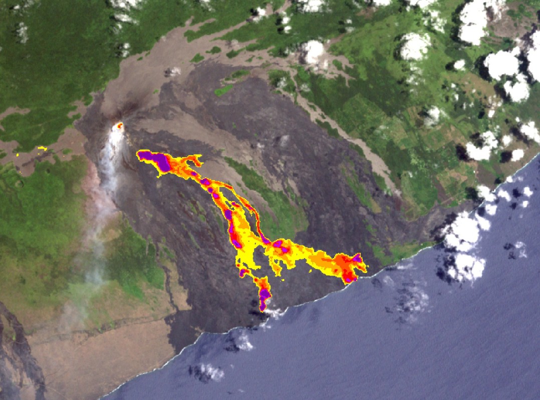
Signal recorded by the thermal infrared channel of Landsat 7 for part of Hawaii Big Island (left) and overlay of active lava flows derived from the thermal infrared channel with true-color composite and (right).