Lesson 4: Advanced remote sensing methods

1. Retrieval and preparation of data

This lesson relies on ASTER and WorldView-1 imagery as well as on the extent shapefiles for each task. The imagery is not freely available from the internet. It has to be purchased, alternatively it may be downloaded from this web site. One has to emphasize that the imagery may only be used for the purpose of this training course and for nothing else.

Access GIS and RS data sources
Download training data for the Pamir

1. Generation of a high-resolution DEM from WorldView-1 stereo imagery

We will first generate a DEM for the Rivakkul Lake in the Pamir of Tajikistan from a stereo pair of WorldView-1 images. In contrast to the lessons before, it is essential to use geometrically uncorrected data: the distortions due to mountainous terrain and different angles of observations are important for a successful DEM extraction. In order to avoid very long computing times, the extent of the new DEM will be constrained to the polygon gv_extent2.shp.

Stereo matching of satellite imagery cannot be performed using standard GIS software like ArcGIS or GRASS GIS. Specialized Remote Sensing software is required, e.g. ERDAS Imagine or PCI Geomatica. In the present course we will use ERDAS Imagine 2010.

1. Start the Leica Photogrammetric Suite (LPS) from the Toolbox menu. The LPS Project Manager will open.
2. Create a new project (block file *.blk). Choose Orbital Pushbroom as Geometric Model Category and QuickBird/WorldView as Geometric Model. You can leave the default values for the Reference Coordinate System and the Vertical Units unchanged. Set the Average Elevation to 4000 m and then press OK.

   
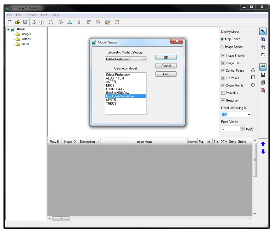
   Dialog box for the choice of Geometric Model Category and Geometric Model.

3. Add the two WorldView-1 images. They represent a stereo pair taken from two different locations. The images can be matched in order to produce a DEM. Since the internal parameters of the sensor and the orbital parameters of the images (altitude, orientation) are known, it is not required to set Ground Control Points (GCPs), even though good GCPs could improve the accuracy of the resulting DEM. Without orbital information available, GCPs would be required.

   
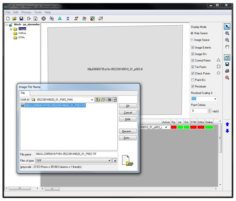
   Adding the WorldView images to the LPS project.

4. Looking at the lower part of the LPS Project Window, you will see green and red field associated to the two images. Green fields mean that the respective task is already done, red fields mean that it still has to be done. Internal (Int.) and external (Ext.) orientation have been taken from the image metadata. Pyramids (Pyr.), helping to speed up zooming of the images, still have to be created just by clicking on the respective red fields.

   
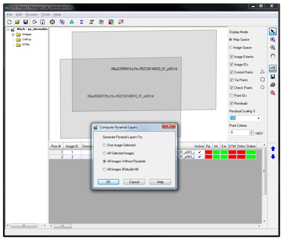
   Dialog box for the creation of pyramid layers.

5. The DTM field is still red, meaning that no DTM (or DEM) was yet created from the pair of images. To generate the DEM, choose Process - DTM Extraction - Classic ATE from the menu bar of the LPS Project Manager.
6. In the DTM Extraction window, choose an appropriate cell size fror the DEM and specify a file name. In general, the cell size should be at least twice that of the original image, but experience has shown that a factor of four or eight usually produces better results. In our case, it is sufficient to choose a cell size of 10 m. It is also possible to select 3D Shape from DTM Type. This would produce an irregular cluster of points which can later be interpolated to a raster, e.g. in ArcGIS or GRASS GIS. Under Advanced Properties, choose the file gv_extent2.shp as Extent. Set the Horizontal Projection to the UTM Zone 43 North (WGS84) and leave the remaining parameters unchanged. Start the DEM Generation by pressing Run in the DTM Extraction Window.

   
   DEM Extraction with LPS - main dialog box (top) and Advanced Properties dialog box (right bottom).

7. After completion of the DEM, load it into ArcGIS and create a hillshade in order to evaluate its general quality. You can compare the newly generated DEM to the SRTM DEM in order to figure out the differences.

   
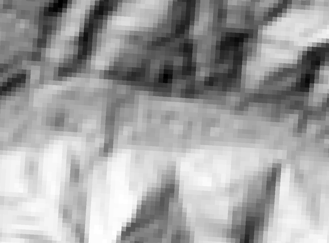
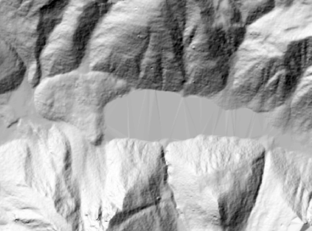
   Hillshades created from the SRTM DEM (approx. 90 m cell size; left), the ASTER GDEM (approx. 25 m cell size; middle) and the DEM created from the stereo pair of WorldView images (10 m cell size; right).

8. Finally, try to drape the hillshade over the DEM in order to get a realistic oblique view of Rivakkul. You can use ArcScene to do so. You can also try to drape an ASTER composite image over the DEM (you have to proceed with the first step of the next task to create an ASTER composite image).

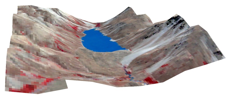
Oblique views of Rivakkul with hillshade (left) and ASTER composite (right) draped over the DEM.
View air photo from approx. the same perspective.

In the DEM Extraction window of the LPS, you could also produce an orthoimage i.e, remove geometric distortions of the original imagery. Only orthoimages allow for an overlay with other images, maps or DEMs. All the images used in the other lessons of this course were already provided as orthoimages, so that this fundamental preprocessing step was not necessary.

2. Supervised classification of ASTER imagery

The information provided by satellite imagery often requires generalization for further processing. Such a generalization can be performed by organizing the image pixels into classes, e.g. vegetation, rock, lakes, glaciers etc. One way to classify images is the NDVI, which was already introduced in Lesson 1.

Another way to classify remotely sensed data is the Unsupervised classification: an algorithm is used to organize the image pixels into a user-defined number of classes, based on the image statistics. In practice, this method is usually not very useful. Instead, it makes more sense that the user defines so-called training areas (e.g. clearly recognizable glaciers, lakes, forests etc.). The computer program then uses those training areas for defining the criteria for the classification. The advantage of this method is that the user can choose which classes she or he wants to distinguish, usually resulting a a more reasonable classification. We will do such a Supervised classification of a false colour composite ASTER image of part of the Tajik Pamir. Even though also ERDAS Imagine offers functionalities for supervised classification, we will use ArcGIS 10.

1. Create an ASTER composite image from the bands V3N, V2, and V1 and clip the result to the extent of the shapefile gv_extent1.shp.

   
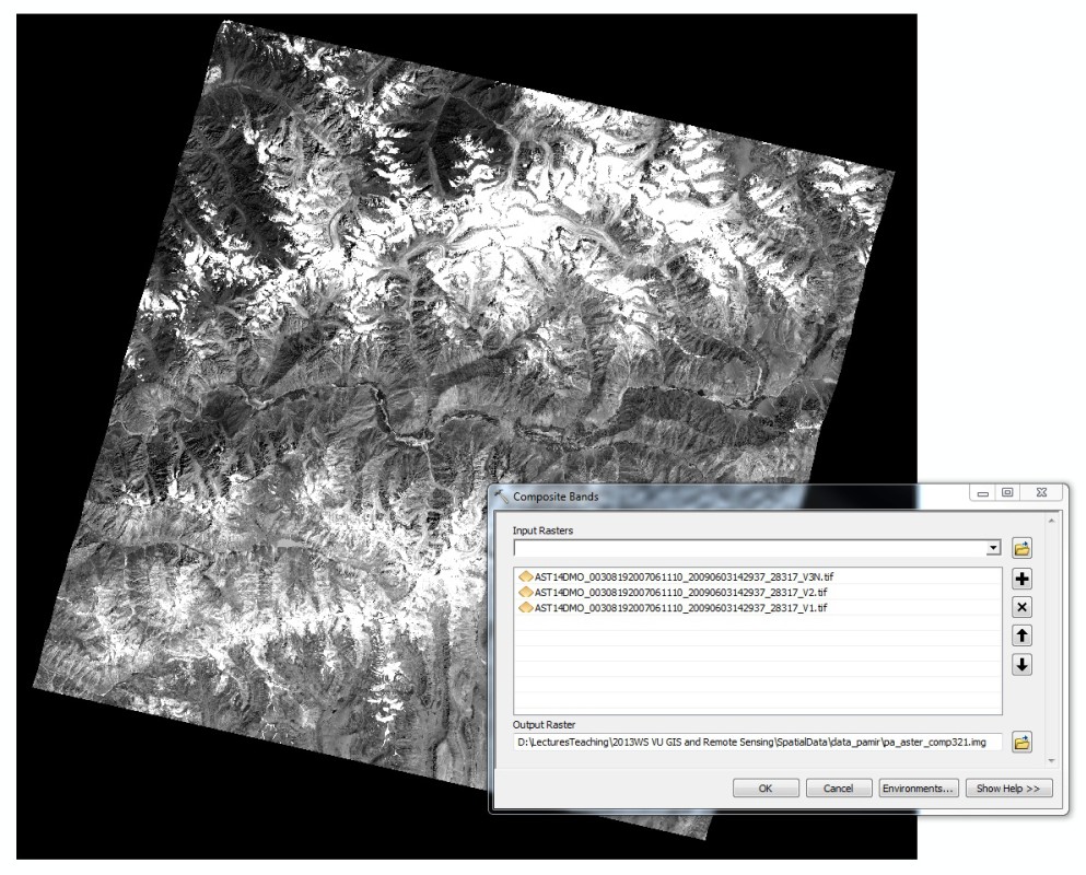
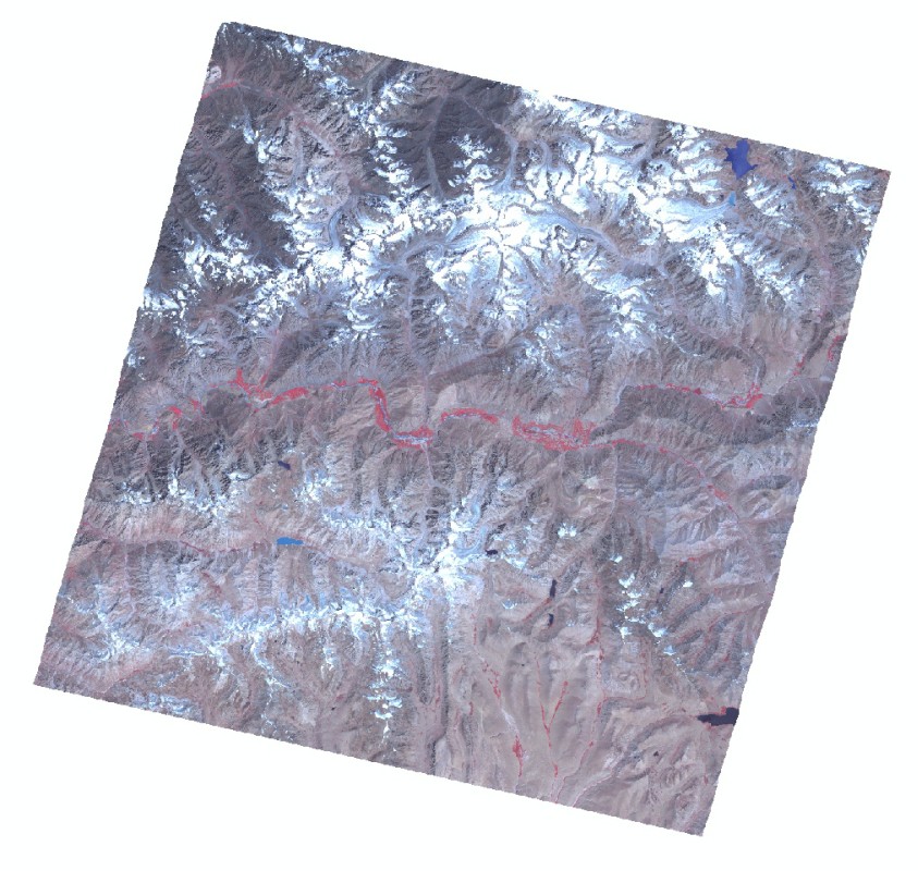
   Creation of a false-colour composite image of three ASTER channels.

2. Load the Image Classification toolbar into your ArcMap project and select the Draw Polygon option.
3. Next, you have to define so-called training areas which are later used to assign each pixel to a certain class, based on the correspondence of the pixel value to the pixel values representing the training areas of each class. First, choose a clearly recognizable lake in the image and draw a polygon within the lake, taking care that only such pixels really part of the lake are within the polygon. Do the same for some more lakes in order to compile a representative sample. The Training Sample Manager will open automatically and a class will be created for each polygon you draw. Finally, select all the classes and merge them into one class (Merge training samples in the menu of the Training Sample Manager. Rename the resulting class to Lakes.
4. Repeat the previous step for glaciers, snow, fields, debris and rocks.

   
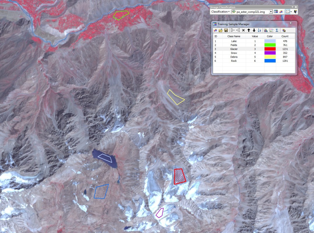
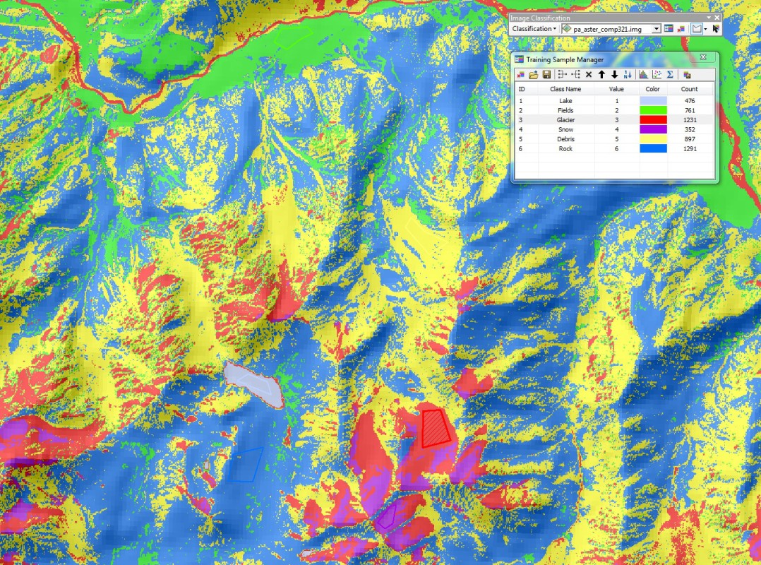
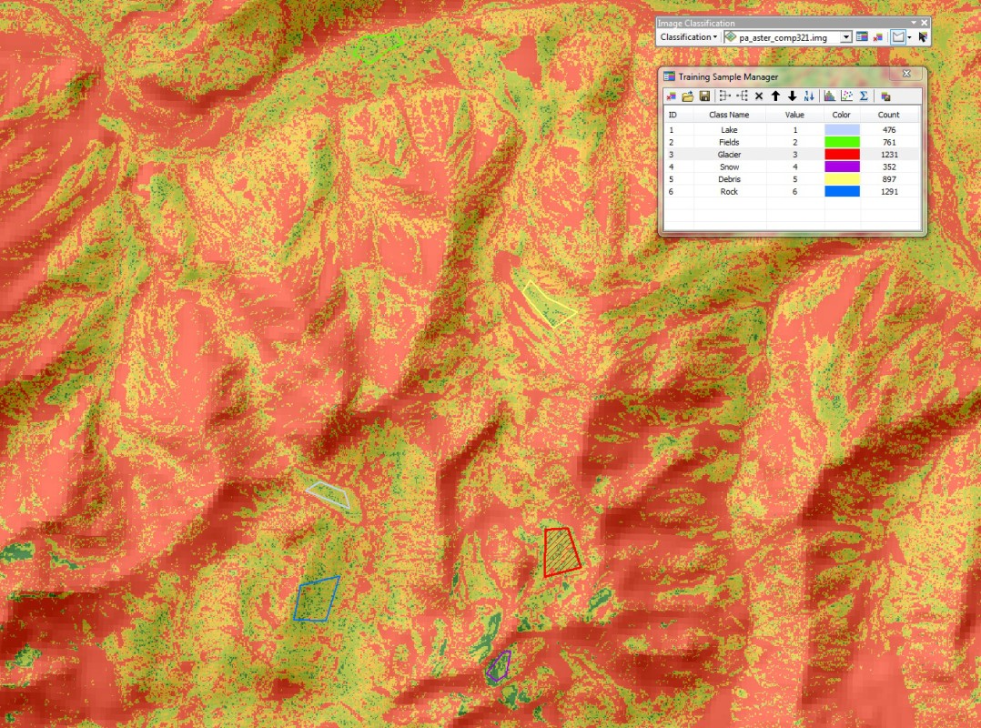
   Training areas and Training Sample Manager.

5. Now you have a set of five signature classes, each connected to certain ranges of pixel value combinations. Create a signature file (menu of the Training Sample Manager) to save the signatures of each class.

   
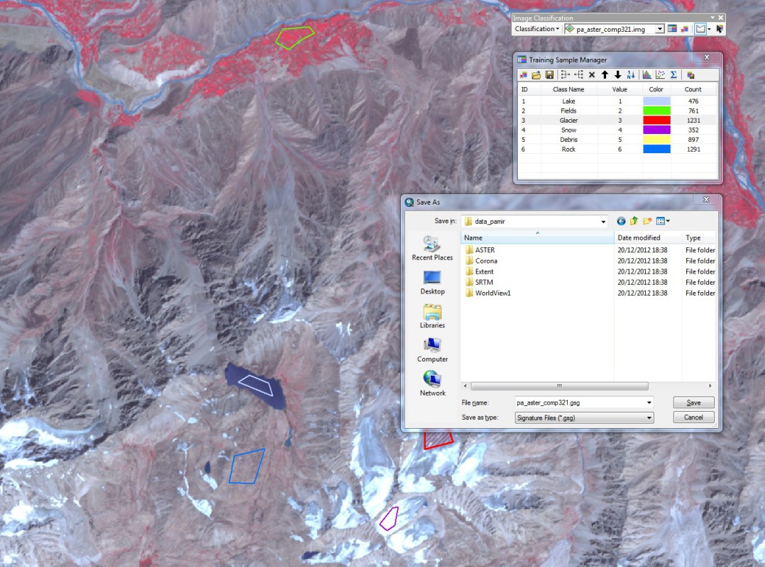
   Saving the training areas to a signature file.

6. Choose Maximum Likelihood Classification from the Image Classification toolbar. Specify the Input raster bands, Signature file, Output classified raster and and Output confidence raster and execute the classification.

   
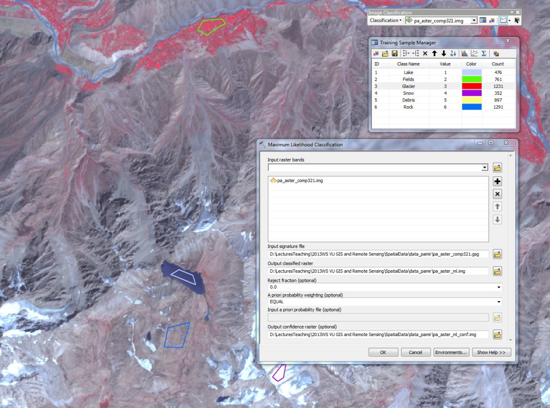
   Dialog box for performing a Maximum Likelihood Classification.

7. You will probably see that the fields in the valley bottom and the snow on the mountains were classified in a satisfactory way, as were some of the lakes. In contrast, the distinction between glaciers, rock and debris did not work properly since the difference of the pixel values of the channels used is not clear enough. In such cases, other channels or other data have to be used, or the features have to be mapped manually.

   
   Classified (left) and confidence (right) rasters.

8. You can also try the other classification methods offered by the Image Classification toolbar and compare the results to those yielded by the Maximum Likekihood Classification.

Also ERDAS Imagine offers a functionality to perform a supervised image classification. You can try this functionality alternatively and then compare the results yielded by the two different software packages.

1. Load the clipped ASTER composite image into ERDAS Imagine (with the command Open).
2. Choose the Signature Editor from the Raster - Supervised menu. It allows you to define different classes, based on polygons drawn in corresponding areas of the image.
3. In order to define the classes, you have to create an Area of Interest (AOI) layer for each class. Create such a layer via the New - 2D Layer - AOI Layer menu (accessible from the button in the very upper left corner of the ERDAS Imagine window).
4. Now, select Polygon from the Drawing menu. Choose a clearly recognizable lake in the image and draw a polygon within the lake, taking care that only such pixels really part of the lake are within the polygon. Do the same for some more lakes in order to compile a representative sample. Then, select all of the polygons you have drawn.
5. In the Signature Editor, press Create New Signature(s) from AOI, and the statistics of the pixels coinciding with your polygons will be loaded and displayed. If you have drawn more than one polygon, one class will be created for each polygon. In this case, merge the classes and then remove the classes for each single polygon. You can rename the class from Class * to Lakes.
6. Repeat the tasks 5. and 6. for snow, glaciers, rock and vegetation.
7. Now you have a set of five signature classes, each connected to certain ranges of pixel value combinations. Save this setting as signature file *.sig.
8. Choose Supervised Classification from the Raster - Supervised menu. Specify the Input, Signature and Output files and start the classification process by pressing OK.
9. Open the classified image file in ArcGIS. You will probably see that the vegetated areas in the valley bottom were classified in a satisfactory way, as were some of the lakes. In contrast, the distinction between glaciers and rock did not work properly since the difference of the pixel values of the channels used is not clear enough. In such cases, other channels or other data have to be used, or the features have to be mapped manually.

In contrast to the pixel-based classification methods, also object-based approaches exist. They make use not only of pixel values, but also of neighbourhood relations between pixels and image textures. Object-based image classification is more complex than pixel-based classification and requires specialized software, but is also more powerful.

Access introduction to object-based image classification

3. Introduction to the basics of laser scanning (LiDAR)

Laser scanning or Lidar (Light detection and ranging) is an active Remote Sensing method measuring the travel time of the laser beam from the sensor to the reflecting surface and back as well as the reflected intensity. High-resulution DEMs, reaching far into the sub-meter scale, can be generated by this technique. One may distinguish between airborne laser scanning (sensor fixed at an airplane or helicopter) and terrestrial laser scanning (sensor placed e.g. at the opposite slope or on a mountain top). Conversion of the raw point clouds provided by laser scanners to usable raster DEMs is not trivial and requires some know-how.

Since laser scanners are not fixed to satellites, there are no worldwide archives of Lidar data. Instead many national and regional agencies hold Lidar DEMs. Some of these agencies charge high prices for the data, others offer them at reduced prices or even for free for scientific or educational use. The government of South Tyrol / Alto Adige (Northern Italy) offers its Lidar DEM for the entire province for free.

Access DEM of South Tyrol more information about Lidar

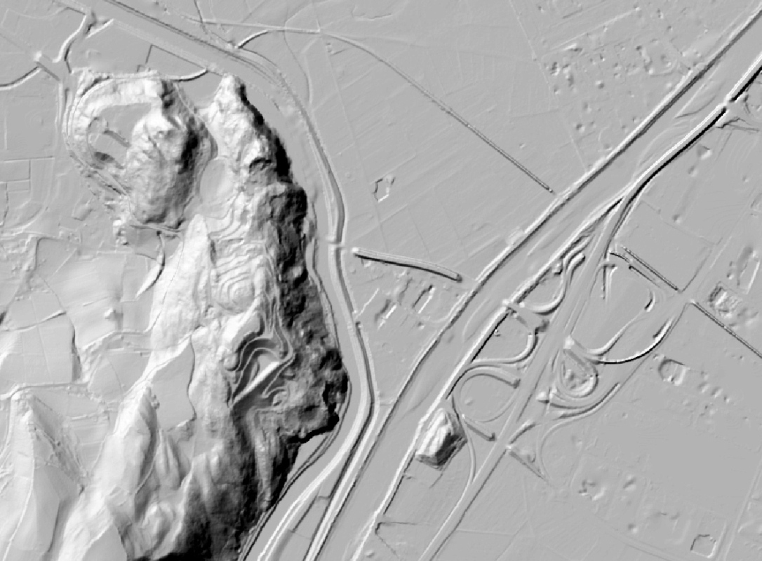
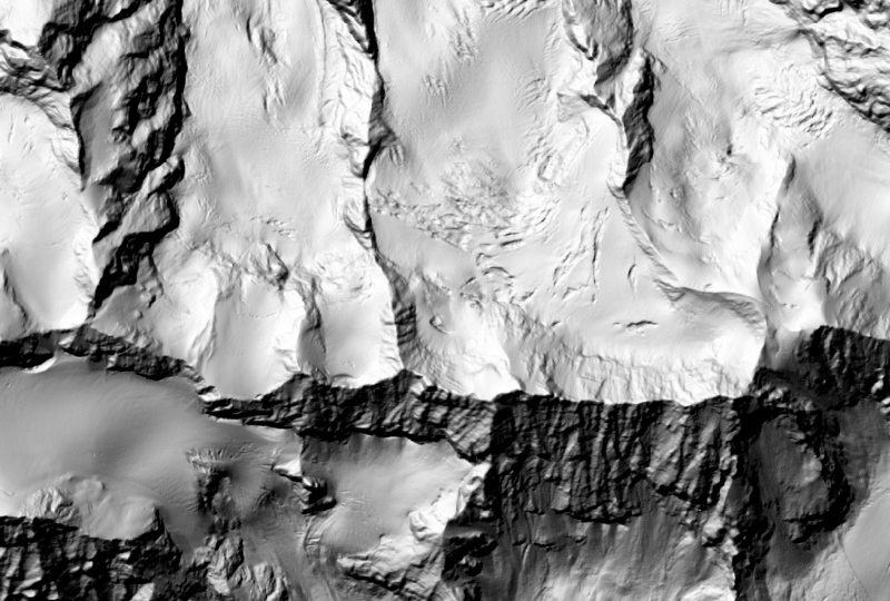
Laser scan DEMs for South Tyrol (cell size: 2 m): part of the Etsch Valley south of Bozen with the highway entrance Bozen-Süd (left), Ortler Mountains (right), source: Autonome Provinz Bozen - Südtirol, Abteilung Informationstechnik.

4. Introduction to the basics of radar remote sensing (SAR)

Like Lidar, SAR (Synthetic Aperture Radar) is an active remote sensing method. It is particularly useful for collecting information on areas frequently covered by clouds not accessible to passive RS methods working with visible or infrared radiation. The interpretation of radar imagery is non-trivial.

A field of particular interest for the Applied Geosciences is radar interferometry (InSAR): the phase shift of the radar waves is measured in order to derive the distance between the sensor and the terrain and to produce DEMs. Differential radar interferometry (DinSAR) even goes one step further and allows the identification of changes in elevation (subsidence, ground displacemnts). Radar sensors may be fixed to airplanes, space shuttles (e.g. SRTM) or satellites. In the tutorial below, the focus is put on the Canadian satellite RADARSAT, but other radar sensors exist or have existed, e.g. those of the ERS satellites, ASAR or TERRASAR-X, operated by the European Space Association (ESA), or the SAR sensor of the Japanese JERS satellite.

Access more information on radar interferometry (InSAR)